볼록 조합(Convex Combination)의 이론과 응용

1 Introduction

볼록 조합(Convex Combination)은 수학, 최적화 이론, 머신러닝에서 핵심적인 역할을 하는 개념이다. 본 문서는 볼록 조합의 수학적 정의부터 시작하여, 기하학적 해석, 최적화 이론에서의 중요성, 그리고 머신러닝 및 다양한 응용 분야에서의 활용까지를 체계적으로 다룬다.

볼록 조합은 단순히 점들의 가중 평균을 넘어서, 볼록 최적화의 전역 최솟값 보장, 커널 방법론의 이론적 기반, 그리고 정규화 기법의 설계 원리 등 현대 데이터 과학의 여러 핵심 개념과 깊이 연결되어 있다.

2 Mathematical Foundations

2.1 볼록 조합의 정의

Definition 1.1 (Convex Combination): \(k\)개의 점(벡터) \(x_1, x_2, \ldots, x_k \in \mathbb{R}^d\)가 주어졌을 때, 이들의 볼록 조합(convex combination)은 다음과 같이 정의된다:

\[x = \sum_{i=1}^k \alpha_i x_i\]

여기서 계수 \(\alpha_i\)는 다음 두 조건을 만족해야 한다:

1. 비음 조건 (Non-negativity): \[\alpha_i \geq 0 \quad \text{for all } i = 1, \ldots, k\]

2. 정규화 조건 (Normalization): \[\sum_{i=1}^k \alpha_i = 1\]

이러한 조건들은 결과 점 \(x\)가 원래 점들의 가중 평균(weighted average)이 되도록 보장한다.

2.2 Affine Combination과의 관계

볼록 조합은 affine combination의 특수한 경우이다:

• Affine Combination: \(\sum_{i=1}^k \alpha_i = 1\) (비음 조건 없음)
• Convex Combination: \(\sum_{i=1}^k \alpha_i = 1\) AND \(\alpha_i \geq 0\) (비음 조건 추가)

Affine combination은 점들이 정의하는 affine subspace의 모든 점을 표현하는 반면, convex combination은 그 중에서도 “점들 사이”에 위치하는 점들만을 표현한다.

2.3 Carathéodory’s Theorem

Theorem 1.1 (Carathéodory): \(\mathbb{R}^d\) 공간에서 어떤 점들의 convex hull에 속하는 모든 점은 최대 \(d+1\)개 점의 convex combination으로 표현할 수 있다.

이 정리는 실용적으로 매우 중요하다. 예를 들어, 3차원 공간(\(d=3\))에서는 어떤 점이든 최대 4개의 점만으로 convex combination을 구성할 수 있다는 의미이다. 이는 계산 복잡도를 크게 줄여준다.

3 Geometric Interpretation

3.1 저차원 공간에서의 시각화

3.1.1 두 점의 경우: 선분

두 점 \(x_1, x_2 \in \mathbb{R}^d\)의 convex combination은:

\[x = \alpha_1 x_1 + \alpha_2 x_2, \quad \alpha_1 + \alpha_2 = 1, \quad \alpha_1, \alpha_2 \geq 0\]

\(\alpha_1 = 1 - t\), \(\alpha_2 = t\) (단, \(t \in [0,1]\))로 parametrize하면:

\[x(t) = (1-t)x_1 + tx_2\]

이는 두 점을 잇는 선분(line segment)의 매개변수 방정식이다:

• \(t = 0\): \(x = x_1\) (시작점)
• \(t = 1\): \(x = x_2\) (끝점)
• \(t = 0.5\): \(x = \frac{1}{2}(x_1 + x_2)\) (중점)

3.1.2 세 점의 경우: 삼각형

세 점 \(x_1, x_2, x_3 \in \mathbb{R}^2\)의 convex combination은:

\[x = \alpha_1 x_1 + \alpha_2 x_2 + \alpha_3 x_3, \quad \sum_{i=1}^3 \alpha_i = 1, \quad \alpha_i \geq 0\]

이는 세 점을 꼭짓점으로 하는 삼각형의 내부와 경계에 있는 모든 점을 표현한다. 계수 \((\alpha_1, \alpha_2, \alpha_3)\)는 무게중심 좌표(barycentric coordinates)로 해석된다.

#| label: fig-triangle
#| fig-cap: "세 점의 convex combination으로 생성되는 삼각형"
#| code-fold: true

import numpy as np
import matplotlib.pyplot as plt
from matplotlib.patches import Polygon

# 세 꼭짓점 정의
vertices = np.array([[0, 0], [4, 0], [2, 3]])

# 삼각형 그리기
fig, ax = plt.subplots(figsize=(8, 6))
triangle = Polygon(vertices, alpha=0.3, facecolor='skyblue', edgecolor='navy', linewidth=2)
ax.add_patch(triangle)

# 꼭짓점 표시
ax.plot(vertices[:, 0], vertices[:, 1], 'ro', markersize=10, label='Original Points')
for i, v in enumerate(vertices):
    ax.annotate(f'$x_{i+1}$', xy=v, xytext=(5, 5), textcoords='offset points', fontsize=14)

# 내부의 convex combination 예시
np.random.seed(42)
n_samples = 50
alphas = np.random.dirichlet([1, 1, 1], n_samples)
interior_points = alphas @ vertices

ax.scatter(interior_points[:, 0], interior_points[:, 1], 
          alpha=0.5, s=20, c='orange', label='Convex Combinations')

ax.set_xlim(-0.5, 4.5)
ax.set_ylim(-0.5, 3.5)
ax.set_aspect('equal')
ax.grid(True, alpha=0.3)
ax.legend()
ax.set_title('Convex Combinations of Three Points', fontsize=16)
plt.tight_layout()
plt.show()

3.2 Convex Hull과의 관계

Definition 1.2 (Convex Hull): 점들의 집합 \(S = \{x_1, \ldots, x_k\}\)의 convex hull은 이 점들의 모든 가능한 convex combination의 집합이다:

\[\text{conv}(S) = \left\{ \sum_{i=1}^k \alpha_i x_i \,\Big|\, \sum_{i=1}^k \alpha_i = 1, \, \alpha_i \geq 0 \right\}\]

Convex hull은 \(S\)를 포함하는 가장 작은 convex set이다.

3.3 유한 점 vs. 무한 점의 Convex Set

3.3.1 유한 개의 점

유한한 개수의 점들의 convex hull은 항상 다각형(polygon) 또는 다면체(polytope) 형태이다:

• 2차원: 선분, 삼각형, 사각형, … , \(n\)-각형
• 3차원: 사면체, 피라미드, 프리즘, …

중요: 유한 점들의 convex hull은 곡선 경계를 가질 수 없다. 경계는 항상 직선 선분들로 구성된다.

3.3.2 무한히 많은 점

Convex set의 정의는 무한 개의 점을 포함하는 집합에도 적용된다:

Definition 1.3 (Convex Set): 집합 \(C \subseteq \mathbb{R}^d\)가 convex set이라는 것은, \(C\) 내의 임의의 두 점 \(x_1, x_2 \in C\)에 대해 그들을 잇는 선분 전체가 \(C\)에 포함되는 것이다:

\[\forall x_1, x_2 \in C, \, \forall \lambda \in [0, 1]: \quad \lambda x_1 + (1-\lambda)x_2 \in C\]

무한 점을 포함하는 convex set의 예:

• 원판(Disk): \(\{x \in \mathbb{R}^2 \mid \|x - c\|_2 \leq r\}\)
• 타원체(Ellipsoid): \(\{x \in \mathbb{R}^d \mid (x-c)^T P^{-1} (x-c) \leq 1\}\) (단, \(P \succ 0\))
• 반공간(Halfspace): \(\{x \in \mathbb{R}^d \mid a^T x \leq b\}\)

이러한 집합들은 곡선 경계를 가질 수 있다.

4 Convex Optimization Theory

4.1 Convex Function의 정의

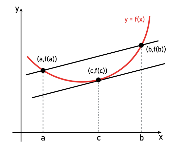
Definition 2.1 (Convex Function): 함수 \(f: \mathbb{R}^d \to \mathbb{R}\)가 convex function이라는 것은, 그 정의역이 convex set이고, 임의의 \(x_1, x_2\)와 \(\lambda \in [0,1]\)에 대해 다음을 만족하는 것이다:

\[f(\lambda x_1 + (1-\lambda)x_2) \leq \lambda f(x_1) + (1-\lambda)f(x_2)\]

기하학적으로, 이는 함수 그래프 위의 임의의 두 점을 잇는 선분이 항상 함수 그래프의 위쪽에 위치함을 의미한다.

Convex Function

4.2 전역 최솟값 보장의 원리

Convex optimization에서 가장 중요한 성질은 다음 정리이다:

Theorem 2.1 (Local-Global Optimality): \(f: \mathbb{R}^d \to \mathbb{R}\)이 convex function이고 \(C \subseteq \mathbb{R}^d\)이 convex set일 때, \(x^* \in C\)가 local minimum이면 global minimum이다.

증명 스케치:

귀류법으로 증명한다. \(x^*\)가 local minimum이지만 global minimum이 아니라고 가정하자. 그렇다면 다음을 만족하는 \(y \in C\)가 존재한다:

\[f(y) < f(x^*)\]

\(C\)가 convex set이므로, \(\lambda \in (0, 1)\)에 대해:

\[x_\lambda = \lambda y + (1-\lambda)x^* \in C\]

\(f\)의 convexity에 의해:

\[f(x_\lambda) \leq \lambda f(y) + (1-\lambda)f(x^*) < \lambda f(x^*) + (1-\lambda)f(x^*) = f(x^*)\]

\(\lambda\)가 충분히 작으면 \(x_\lambda\)는 \(x^*\)의 국소 근방(local neighborhood)에 위치하므로, 이는 \(x^*\)가 local minimum이라는 가정에 모순이다. \(\square\)

실용적 함의: 이 정리는 gradient descent와 같은 local search 알고리즘이 convex optimization 문제에서는 항상 전역 최적해를 찾는다는 것을 보장한다.

4.3 Convex Optimization Problem의 표준형

표준적인 convex optimization problem은 다음과 같이 정식화된다:

\[ \begin{align} \min_{x \in \mathbb{R}^d} \quad & f(x) \\ \text{subject to} \quad & g_i(x) \leq 0, \quad i = 1, \ldots, m \\ & h_j(x) = 0, \quad j = 1, \ldots, p \end{align} \]

여기서: - \(f\): convex objective function - \(g_i\): convex inequality constraint functions - \(h_j\): affine equality constraint functions (\(h_j(x) = a_j^T x - b_j\))

핵심: 제약 조건이 정의하는 feasible region이 convex set을 형성한다.

5 Applications in Machine Learning

5.1 Elastic Net Regularization

5.1.1 배경: Ridge와 Lasso의 한계

선형 회귀에서 두 대표적인 정규화 방법:

• Ridge Regression (L2): \(P_{\text{Ridge}} = \|\beta\|_2^2 = \sum_{j=1}^p \beta_j^2\)
  • 장점: 안정적, 다중공선성 처리
  • 단점: 변수 선택 불가 (모든 계수를 0이 아닌 값으로 축소)
• Lasso Regression (L1): \(P_{\text{Lasso}} = \|\beta\|_1 = \sum_{j=1}^p |\beta_j|\)
  • 장점: 변수 선택 가능 (일부 계수를 정확히 0으로)
  • 단점: 강한 상관관계가 있는 변수 중 임의로 하나만 선택

5.1.2 Elastic Net의 정의

Elastic Net (Zou & Hastie, 2005)은 L1과 L2 페널티의 convex combination을 사용한다:

\[ \min_{\beta \in \mathbb{R}^p} \left\{ \frac{1}{2n}\|y - X\beta\|_2^2 + \lambda\left[(1-\alpha)\frac{1}{2}\|\beta\|_2^2 + \alpha\|\beta\|_1\right] \right\} \]

여기서: - \(\lambda > 0\): 전체 정규화 강도 (regularization strength) - \(\alpha \in [0, 1]\): L1과 L2의 혼합 비율 (mixing parameter)

페널티 항을 다시 쓰면:

\[P_{\text{Elastic Net}} = (1-\alpha) P_{\text{Ridge}} + \alpha P_{\text{Lasso}}\]

\((1-\alpha) + \alpha = 1\)이고 두 가중치가 모두 비음이므로, 이는 완벽한 convex combination이다.

5.1.3 Convex Combination 사용의 필요성

만약 가중치의 합이 1이 아니라면?

예를 들어, \(w_1 P_{\text{Ridge}} + w_2 P_{\text{Lasso}}\) (단, \(w_1 + w_2 \neq 1\))를 사용한다면:

1. 하이퍼파라미터 해석 불가능:
   • \(\lambda\)는 “전체 정규화 강도”를 조절
   • \(\alpha\)는 “L1 vs. L2의 상대적 비율”을 조절
   • 이 두 역할이 명확히 분리되지 않으면, 하이퍼파라미터 튜닝이 극도로 복잡해진다.
2. 수학적 일관성 상실:
   • \(\alpha = 0\): Pure Ridge
   • \(\alpha = 1\): Pure Lasso
   • \(\alpha \in (0, 1)\): 두 방법의 “보간(interpolation)”
   • 이러한 깔끔한 해석은 convex combination에서만 가능하다.
3. Convexity 보존:
   • Ridge와 Lasso 페널티는 모두 convex function
   • Convex function들의 convex combination은 다시 convex
   • 따라서 Elastic Net은 convex optimization 보장

실증 연구: Zou & Hastie (2005, JRSSB 67(2):301-320)는 Elastic Net이 다음 상황에서 우수함을 보였다: - \(p > n\) (변수 개수가 샘플 수보다 많을 때) - Grouped selection 필요 시 (상관된 변수들을 함께 선택)

5.2 Reproducing Kernel Hilbert Space (RKHS)

5.2.1 Hilbert Space의 정의

Definition 3.1 (Hilbert Space): Hilbert space \(\mathcal{H}\)는 다음 조건을 만족하는 벡터 공간이다:

1. 내적(Inner Product): \(\langle \cdot, \cdot \rangle_{\mathcal{H}}: \mathcal{H} \times \mathcal{H} \to \mathbb{R}\) 존재
2. 완비성(Completeness): 모든 Cauchy 수열이 \(\mathcal{H}\) 내의 극한값으로 수렴
3. 벡터 공간: 덧셈과 스칼라 곱 정의

Hilbert space는 유클리드 공간 \(\mathbb{R}^d\)를 무한 차원으로 일반화한 개념이다. 내적이 정의되므로 “길이”, “각도”, “직교성” 개념을 사용할 수 있다.

예시: - \(\mathbb{R}^d\) (유한 차원) - \(L^2[0, 1]\) (제곱 적분 가능한 함수들의 공간, 무한 차원)

5.2.2 RKHS와 Kernel Trick

Definition 3.2 (Reproducing Kernel Hilbert Space): Hilbert space \(\mathcal{H}\)가 RKHS라는 것은, 모든 점 \(x\)에 대해 evaluation functional \(\delta_x: f \mapsto f(x)\)가 bounded linear functional인 것이다.

Moore-Aronszajn Theorem: 모든 positive definite kernel \(K: \mathcal{X} \times \mathcal{X} \to \mathbb{R}\)에 대해, 유일한 RKHS \(\mathcal{H}\)가 존재하며:

\[K(x, x') = \langle \phi(x), \phi(x') \rangle_{\mathcal{H}}\]

여기서 \(\phi: \mathcal{X} \to \mathcal{H}\)는 feature map이다.

5.2.3 Support Vector Machine에서의 활용

Kernel SVM의 dual problem:

\[ \max_{\alpha} \left\{ \sum_{i=1}^n \alpha_i - \frac{1}{2}\sum_{i,j=1}^n \alpha_i \alpha_j y_i y_j K(x_i, x_j) \right\} \]

subject to: \(\sum_{i=1}^n \alpha_i y_i = 0\), \(0 \leq \alpha_i \leq C\)

핵심 아이디어: - 원본 공간 \(\mathcal{X}\)에서는 선형 분리 불가능 - Feature map \(\phi\)를 통해 \(\mathcal{H}\)로 매핑하면 선형 분리 가능 - \(\phi\)를 명시적으로 계산하지 않고, kernel \(K(x, x')\)만으로 내적 계산 - RKHS 이론이 이 과정의 수학적 정당성을 제공

대표 커널: - RBF kernel: \(K(x, x') = \exp\left(-\frac{\|x-x'\|^2}{2\sigma^2}\right)\) (무한 차원 \(\mathcal{H}\)) - Polynomial kernel: \(K(x, x') = (x^T x' + c)^d\)

문헌: - Aronszajn (1950, Trans. AMS 68:337-404): RKHS 이론적 기초 - Schölkopf & Smola (2002): Learning with Kernels, MIT Press

6 Applications in Other Fields

6.1 경제학: Portfolio Theory

6.1.1 Markowitz Mean-Variance Optimization

투자자가 \(k\)개 자산에 투자할 때, 포트폴리오의 기대 수익률과 분산:

\[ \begin{align} \mathbb{E}[R_p] &= \sum_{i=1}^k \alpha_i \mathbb{E}[R_i] \\ \text{Var}(R_p) &= \sum_{i,j=1}^k \alpha_i \alpha_j \text{Cov}(R_i, R_j) \end{align} \]

여기서 \(\alpha_i\)는 자산 \(i\)의 투자 비중이며, 다음 제약을 만족:

• \(\sum_{i=1}^k \alpha_i = 1\) (전체 자본 투자)
• \(\alpha_i \geq 0\) (공매도 금지 시)

이는 전형적인 convex combination이며, 포트폴리오 최적화 문제는 convex optimization이다 (분산 최소화는 convex, 수익률 제약은 linear).

Efficient Frontier: 주어진 기대 수익률에서 분산을 최소화하는 포트폴리오들의 집합은 convex set을 형성한다.

6.2 컴퓨터 그래픽스: Bézier Curves

6.2.1 Linear Interpolation (Lerp)

두 점 \(P_0, P_1\) 사이의 선형 보간:

\[P(t) = (1-t)P_0 + tP_1, \quad t \in [0, 1]\]

이는 convex combination이며, \(t\)에 대한 연속적인 궤적을 그린다.

6.2.2 Bézier Curve

제어점 \(P_0, P_1, \ldots, P_n\)에 대한 \(n\)차 Bézier curve:

\[B(t) = \sum_{i=0}^n \binom{n}{i} (1-t)^{n-i} t^i P_i, \quad t \in [0, 1]\]

Bernstein polynomial \(b_{i,n}(t) = \binom{n}{i} (1-t)^{n-i} t^i\)는:

\[\sum_{i=0}^n b_{i,n}(t) = 1, \quad b_{i,n}(t) \geq 0 \text{ for } t \in [0, 1]\]

따라서 \(B(t)\)는 제어점들의 convex combination이다.

중요한 성질 (Convex Hull Property): Bézier curve는 항상 제어점들의 convex hull 안에 위치한다. 이는 geometric design에서 매우 중요한 성질이다.

#| label: fig-bezier
#| fig-cap: "3차 Bézier curve와 제어점의 convex hull"
#| code-fold: true

import numpy as np
import matplotlib.pyplot as plt
from scipy.special import comb

def bezier_curve(control_points, n_samples=100):
    """Compute Bézier curve from control points"""
    n = len(control_points) - 1
    t = np.linspace(0, 1, n_samples)
    
    curve = np.zeros((n_samples, 2))
    for i, P in enumerate(control_points):
        bernstein = comb(n, i) * (1-t)**(n-i) * t**i
        curve += np.outer(bernstein, P)
    
    return curve

# 제어점 정의
control_points = np.array([[0, 0], [1, 2], [3, 2], [4, 0]])

# Bézier curve 계산
curve = bezier_curve(control_points)

# 시각화
fig, ax = plt.subplots(figsize=(10, 6))

# Convex hull (단순히 제어점들을 순서대로 연결)
from matplotlib.patches import Polygon
hull = Polygon(control_points, alpha=0.2, facecolor='lightblue', 
               edgecolor='blue', linewidth=1.5, linestyle='--', label='Convex Hull')
ax.add_patch(hull)

# Bézier curve
ax.plot(curve[:, 0], curve[:, 1], 'r-', linewidth=2.5, label='Bézier Curve')

# 제어점
ax.plot(control_points[:, 0], control_points[:, 1], 'ko-', 
        markersize=10, linewidth=1, alpha=0.5, label='Control Points')
for i, P in enumerate(control_points):
    ax.annotate(f'$P_{i}$', xy=P, xytext=(5, 5), textcoords='offset points', fontsize=12)

ax.set_xlim(-0.5, 4.5)
ax.set_ylim(-0.5, 2.5)
ax.set_aspect('equal')
ax.grid(True, alpha=0.3)
ax.legend(loc='upper right')
ax.set_title('Cubic Bézier Curve and Convex Hull Property', fontsize=14)
plt.tight_layout()
plt.show()

6.3 확률론: Mixture Distributions

6.3.1 Gaussian Mixture Model (GMM)

\(K\)개의 Gaussian 분포의 convex combination으로 복잡한 분포를 모델링:

\[p(x) = \sum_{k=1}^K \pi_k \mathcal{N}(x \mid \mu_k, \Sigma_k)\]

여기서: - \(\pi_k \geq 0\): 각 component의 mixing coefficient - \(\sum_{k=1}^K \pi_k = 1\): 확률의 정규화 조건

EM 알고리즘: GMM의 파라미터 \(\{\pi_k, \mu_k, \Sigma_k\}\)를 추정하는 데 사용되며, 각 iteration에서 convex combination의 가중치 \(\pi_k\)를 업데이트한다.

응용: - 이미지 segmentation - 음성 인식 - 이상치 탐지

7 Conclusion

볼록 조합(Convex Combination)은 단순한 수학적 정의를 넘어, 현대 최적화 이론, 머신러닝, 그리고 다양한 응용 분야의 핵심 개념으로 자리잡고 있다.

핵심 Takeaways:

1. 수학적 우아함: 가중치의 비음성과 합=1 조건은 결과가 원래 점들의 “사이”에 위치함을 보장한다.

2. 최적화 이론의 기초: Convex optimization에서 local minimum = global minimum이라는 강력한 보장은 convex function과 convex set의 성질에서 비롯된다.

3. 머신러닝의 설계 원리: Elastic Net의 정규화, RKHS 기반의 커널 방법론 등 핵심 기법들이 convex combination을 활용한다.

4. 학제간 응용: 경제학의 포트폴리오 이론, 컴퓨터 그래픽스의 곡선 설계, 확률론의 혼합 분포 등 광범위한 분야에서 활용된다.

5. 계산적 효율성: Carathéodory’s theorem은 고차원에서도 제한된 수의 점만으로 convex combination을 표현할 수 있음을 보장하여, 실용적 알고리즘 설계를 가능하게 한다.

볼록 조합의 이해는 현대 데이터 과학과 최적화 이론을 깊이 있게 학습하는 데 필수적인 기초를 제공한다.

8 References

8.1 주요 참고문헌

• Aronszajn, N. (1950). Theory of Reproducing Kernels. Transactions of the American Mathematical Society, 68(3), 337-404.

• Boyd, S., & Vandenberghe, L. (2004). Convex Optimization. Cambridge University Press.

• Schölkopf, B., & Smola, A. J. (2002). Learning with Kernels: Support Vector Machines, Regularization, Optimization, and Beyond. MIT Press.

• Zou, H., & Hastie, T. (2005). Regularization and Variable Selection via the Elastic Net. Journal of the Royal Statistical Society: Series B (Statistical Methodology), 67(2), 301-320.

• Markowitz, H. (1952). Portfolio Selection. The Journal of Finance, 7(1), 77-91.

8.2 Appendix: Mathematical Proofs

8.2.1 Proof of Carathéodory’s Theorem

Theorem: 점 \(x \in \text{conv}(S)\) (단, \(S \subset \mathbb{R}^d\))는 \(S\)의 최대 \(d+1\)개 점의 convex combination으로 표현 가능하다.

증명: \(x\)가 \(k > d+1\)개 점 \(x_1, \ldots, x_k\)의 convex combination이라 가정:

\[x = \sum_{i=1}^k \alpha_i x_i, \quad \sum_{i=1}^k \alpha_i = 1, \quad \alpha_i > 0\]

\(k > d+1\)이므로, 벡터 \(\{x_1, \ldots, x_k\} \subset \mathbb{R}^d\)는 선형 종속이다. 따라서:

\[\sum_{i=1}^k \beta_i x_i = 0\]

for some \(\beta_i\) not all zero, with \(\sum_{i=1}^k \beta_i = 0\).

\(\lambda = \min_{i: \beta_i > 0} \frac{\alpha_i}{\beta_i}\)라 하면, \(\alpha_i' = \alpha_i - \lambda\beta_i \geq 0\)이고, 적어도 하나의 \(\alpha_j' = 0\)이다.

\[x = \sum_{i=1}^k \alpha_i' x_i\]

는 \(k-1\)개 점의 convex combination이다. 귀납적으로 반복하면 \(d+1\)개 이하로 줄일 수 있다. \(\square\)